Machine Learning for Static Analysis of Malware – Expansion of Research Scope

Introduction

The work presented in this blog post is that of Ewan Alexander Miles (former UCL MSci student) and explores the expansion of scope for using machine learning models on PE (portable executable) header files to identify and classify malware. It is built on work previously presented by NCC Group, in conjunction with UCL’S Centre for Doctoral Training in Data Intensive Science (CDT DIS), which tackles a binary classification problem for separating malware from benignware [1]. It explored different avenues of data assessment to approach the problem, one of which was observations on PE headers.

Multiple models were compared in [1] for their performance in accurately identifying malware from a testing dataset. A boosted decision tree (BDT) classifier, using the library XGBoost, was found to be most performant, showing a classification accuracy of 98.9%. The PE headers of files, both malicious and benign, were pre-processed into inputs made available to the BDT; following this, the model’s hyperparameters were tuned to improve model accuracy. This same methodology was applied to other models and the results compared, also using the model precision, recall and area under the ROC curve for assessment.

Here, a ‘deep dive’ is conducted on the XGBoost BDT to assess certain features of its training method, along with the robustness and structure of its input datasets. Broken down into four key aspects, this entails studying:

• Whether the model receives enough training statistics, or whether there is room for improvement when a larger dataset is used for training;
• The importance of different PE header features in the model’s training;
• Model performance with various sampling balances applied to the dataset (e.g. weighted heavily with malware);
• Model robustness when trained on data originating from older or newer files (e.g. training with files from 2010, testing on files from 2018).

These all help to develop an understanding of the model’s ‘black box’ process and present opportunities for model improvement, or its adaptation to different problems. Model accuracy, precision, recall, training time and area under the ROC curve are used in its assessment, with explanations given as to the real outputs they present.

What are PE Headers?

PE stands for portable executable – these are files with extensions such as .exe, .dll and .sys. It is a common format for many programs on the Windows OS; in fact, most executable code on Windows is loaded in PE format, whether it be benign or malicious. In general, PEs encapsulate the information necessary for Windows to manage the executable code.

The PE structure is comprised of a Header and a Section; the image below gives a full exploration of a PE:

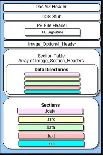
In this analysis, only the header is of interest. It contains different fields of metadata that give an idea of what the entire file looks like. A couple of examples include ‘NumberOfSections’, which is self-explanatory, and the ‘TimeDateStamp’ which is supposed to reference the time of file creation using an ISO Datestring. The latter is used later as a critical element of this investigation.

PE Headers are commonly used in malware analysis [2] [3]. From a machine learning perspective, these PE Header fields can be extracted to form a dataset for model training. These fields form feature inputs for a model that can go on to perform binary classification – in this case, classifying the file as benignware or malware.

With malware sourced from popular file sharing website VirusShare, alongside benign files extracted from Windows OS programs, such as Windows Server 2000, Windows Package Manager and Windows 10 itself, the PE Header dataset was built. After performing a train-test split, the training dataset comprised of 50564 files, with an approximate balance of 44% malware to 56% benignware. Likewise, the test dataset comprised of 11068 files, with an approximate balance of 69% malware to 31% benignware.  A total of 268 input features were used in the dataset, all extracted from the PE headers, with an encoded one-hot labelled ‘IsMalware’ used for prediction.

Precision vs. Recall vs. Accuracy

Before discussing XGBoost’s training and performance on this data, it is worth understanding what each model output represents in terms of what needs to be achieved. The assumed goal here is to be able to correctly identify malware from a set of unlabelled files consisting of both malware and benignware. People familiar to the machine learning process will know about confusion matrices, which can be used to graphically represent binary classification outcomes. A typical binary classification confusion matrix will look like this:

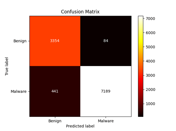
This matrix shows four outcomes side-by-side. True positives, where the model classifies malware as malware, are on the bottom right. True negatives, likewise, are on the top left, and represent the model classifying benignware as benignware. The objective of model improvement can be to reduce the other two outcomes – false negatives, where the model classifies malware as benign (bottom left) and false positive, where the model classifies benignware as malicious (top right). It is intuitive that the preferred outcome is reducing false negatives, where malware is classified as benign.

As such, multiple assessment metrics are used. Precision measures the number of true positives out of the total number of positives:

Thus, here, precision can be thought of as a measure of how many files are correctly labelled as malware out of all the files that are labelled malware. In an ideal world this is 100% – all the files labelled as malware are indeed malware.

What this doesn’t take into consideration is that the number of files labelled as malware might not be equal to the total number of malware files in the dataset! For example, if there are 100 malware and 100 benign files in the dataset and 60 are predicted to be malware, and these 60 are all actually malware, the model outputs 100% precision. However, in this case, it missed 40 malware files. Precision can therefore also be a measure of how much false positives have been reduced – high precision means a low false positive rate.

Recall is in some ways the opposite here, measuring the number of true positives out of the total number of malware files:

So recall is essentially the percentage of malware files labelled correctly. On the other hand, what this doesn’t account for is the false positive rate. Assume there are again 100 malware and 100 benign files in the dataset and 120 are predicted to be malware. These 120 files cover all 100 malware files and 20 benign files. As all malware files are correctly labelled, the model recall is 100%, but it doesn’t register the fact that 20 benign files have been incorrectly labelled as malware. Recall can therefore also be a measure of how much false negatives have been reduced – high recall means a low false negative rate.

Accuracy is less relevant as it doesn’t reflect the dataset’s balance:

Essentially it answers, ‘how often is the prediction correct?’. Now assume a dataset of 10 benign files and 90 malware files. Predicting they are all malware gives an accuracy of 90%, which is very misleading because it completely disregards the benign files.

Knowing what these represent and co-ordinating that with the overall goal is important. If the main goal is to correctly label all malware, it could be assumed that it is acceptable (with a high enough precision) to incorrectly label benignware as malware rather than the other way around. This is a ‘better safe than sorry’ approach, where more research can be done on the false positives afterward. In this circumstance, a higher recall is favoured, reducing the number of malware files falsely labelled as benignware – the false negatives.

Training Statistics

After first training a model and receiving the initial results, something worth investigating almost immediately is the dataset size. Are there enough training statistics for the model to output the best possible results, or might the model benefit from more data to train on?

This can be examined by varying the number of training statistics fed to the model, while keeping the test dataset the same. As the model is fed more and more data in each successive training, its performance is assessed. If a plateau is seen, then that means feeding the model a larger training dataset may be making no difference.

The XGBoost already established in [1], using an even larger dataset than that described above, output the following performance:

Metric	Result (fraction, not %)
Accuracy	0.978
Recall	0.980
Precision	0.970

The first objective was to show that the model could be as performant with the newer, slightly smaller dataset. Following this, the dataset was randomly under-sampled to continuously smaller sizes, with the model performance evaluated at each point. Specifically, the dataset was reduced to 0.1% of its original size, with this incremented by 0.1% intervals until it was 1% of the original size. Following this, it was increased to 2% of its original size, and incremented in 2% intervals until eventually 100% of the dataset was trained on. The results are shown below:

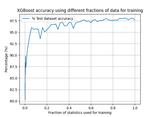
Here, the metric accuracy is used, as it is sufficient to give a blanket idea of model performance. A plateau begins to form when only 20% of the training statistics are used, and it is certain that by a dataset size of 50%, very little increase in performance is achieved by using more data. Remember that only the training dataset is reduced in size, with the model testing on the full 11068 files at each stage.

This confirmed that the model was being fed more than enough training statistics and that, in fact, there was room for training time improvement by reducing the dataset size while bearing only a very small reduction in performance. It also set a baseline that for future analyses, at least 20% of the data should be used when downsampling, to avoid bias in the results from lack of training statistics.

There is still room for improvement on these findings: all metrics (precision, recall) should be examined in future. Furthermore, the dataset could be proportionately sampled to maintain the malware/benign balance, or alternatively different balances should be applied in conjunction with the downsampling.

Feature Importance

To this point, the training dataset comprised of files with 268 input features, all extracted from the PE headers. The next aspect of the training worth testing was whether all of these features were necessary to produce a high-performing model, and what effect removing some of them would have on the training.

A ‘recursive drop’ method was used to implement these tests. The model was trained using all 268 input features, then each input feature was ranked using a function provided by the scikit-learn library, called feature_importances_. It ranks the input features by ‘the mean and standard deviation of accumulation of the impurity decrease within each tree’; more information can be found on it by reading the documentation [4].

Following this, the two least important features were dropped from the dataset and training was conducted using the set now comprised of 266 features. All features were kept in the testing dataset. This was repeated, reducing the number of features by 2 each time, until only 2 features are trained on. The model was evaluated each time a new set of features was implemented. The precision, recall and accuracy all presented similar results:

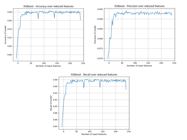
The above show that an alarmingly small number of features can be used in model training to still achieve essentially the same performance, with about 30 input features appearing almost as performant. The feature names were registered at each stage of the recursive drop; as such, the 30 most relevant input features are known to be (ordered left-to-right, moving down):

Magic	MajorLinkerVersion	MinorLinkerVersion
SizeOfUninitializedData	ImageBase	FileAlignment
MajorOperatingSystemVersion	MajorImageVersion	MinorImageVersion
MajorSubsystemVersion	SizeOfImage	SizeOfHeaders
CheckSum	SubSystem	DllCharacteristics
SizeOfStackReserve	SizeOfHeapReserve	NumberOfSections
e_cblp	e_lfanew	SizeOfRawData0
Characteristics0	Characteristics1	Misc2
Characteristics2	Misc3	Characteristics3
Characteristics4	Characteristics5	BaseOfData

A conclusion to be drawn from these evaluations is that these features from the PE header files exhibit the most significant differences between malicious and benign files. However, further research should be conducted into these header features individually, or alternatively the same recursive drop method should be investigated with random features dropped each time.

A more interesting observation drawn from this was the effect on model training time, which may uncover a little about the nature of XGBoost’s black box functions:

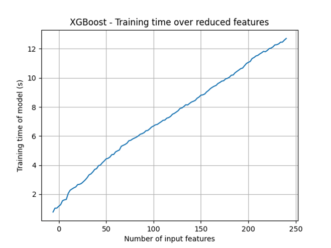
It is visible that the training time using XGBoost decreases in an almost perfectly linear fashion with a reduction of input features. This indicates a strong element of XGBoost’s learning process comes from its looping over input variables, with less time spent looping over fewer inputs. Further investigation here, possibly studying how XGBoost responds to random numbers of inputs and its training time proportionality, is necessary.

Another method of evaluating a model’s performance is the receiver operating characteristic (ROC) curve, which presents the true positive rate as a function of the false positive rate. As the area under an ROC curve tends toward 1, the model is said to be performing better, as it can achieve a very high true positive rate for a very small false positive rate.

A direct comparison of the model using all 268 features with the model using only the 30 above can be made by plotting both ROC curves, which is shown below:

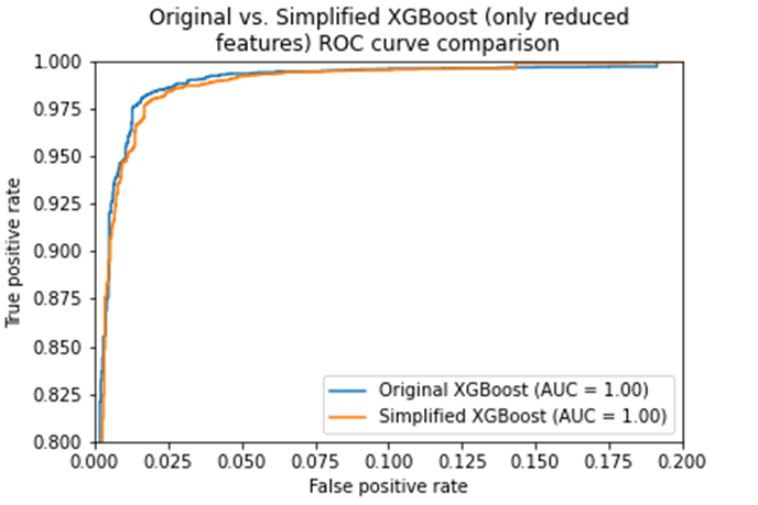
It is clear there is very little difference to be seen between the original (268 feature) XGBoost and the simplified (30 feature) XGBoost. This suggests a massive reduction in training time for very little performance decay.

Dataset Balancing

Machine learning models are known to prioritise identification of different classes when the training dataset is balanced differently [5]. To identify any bias present in the model’s performance, the balance of the dataset was also evaluated. As this was a binary classification problem, achieving a specific dataset balance could be achieved by simply downsampling either the malware or the benignware in the test dataset.

To achieve the desired balance in the dataset, either class was downsampled according to the following equations:  

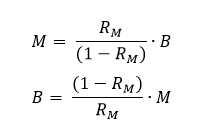
Where M and B are the raw numbers of the malware and benign samples respectively, and R_M is the ‘malware ratio’, given by:

The constraint was also placed that the dataset could not be sampled down to lower than 20% of its original size, as this would re-introduce bias due to lack of training statistics.

Model precision and recall were evaluated after training on increasing amounts of malware present in the dataset; beginning at a balance of 10% malware/90% benignware, the balance of malware was increased in 5% intervals (with the model evaluated each time) up to a dataset formed of 100% malware. The results are below:

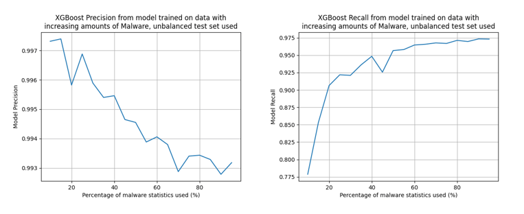
No balance was applied to the test dataset. The graphs above support the conclusion that recall improves in favour of high malware content, meaning the model learns more about how to identify malware from a high balance of it. On the opposing side, the model learns more about how to identify benignware when there is a high balance of benign in the dataset, leading to high precision at low malware content.

The most important conclusion to draw is that this can be used as a tool. By applying specific balances to the training dataset (maintaining enough statistics notwithstanding), a model can be specifically tailored to precision or recall. Again, this will be dependent on the overall goal; a suggestion of this study would be high amounts of malware contributing to a higher recall.

Time Testing

The final aspect of study for this investigation was the effect of selecting training files from a specific time period, to test on newer data. This attempts to yield an understanding of the model’s robustness with time – if it is trained on older data but tested on newer data, is it just as performant? If not, how quickly does it become obsolete, and how often will these models need to be updated and maintained?

The main caveat to the methodology here is that files were selected based on their ‘TimeDateStamp’ header, which should indicate the creation time of the file. This presented two issues:

• This input feature can be modified, falsified, or corrupted
• This input feature can accidentally default to the incorrect datetime

Files dated to the Windows 7 release were a common occurrence, although it is expected some portion of them are incorrect; this was noted in [1]. As such, there is certainly an avenue for improvement on this section for future analyses.

Continuing with this method, further cuts were made in an attempt to improve the dataset. Files dated to years previous to 2000 were removed, as many had suspicious stamps (e.g. dated to epoch, 1 Jan 1970 0x0) and in total they made up a very small fraction of the files. Following this, a split was made such that test files were dated between 2019-2021, and training files began between 2000-2010.

Following this, an ‘expanding window’ method was used. Initially, the model was trained on files from between 2000-2010, tested on files from 2019-2021, and evaluated. Following this, the training set expanded to 2000-2011, and so on until the full training dataset reached years spanning 2000-2018. Note, the test dataset never changed, and no specific balance was applied to either dataset. The results are below:

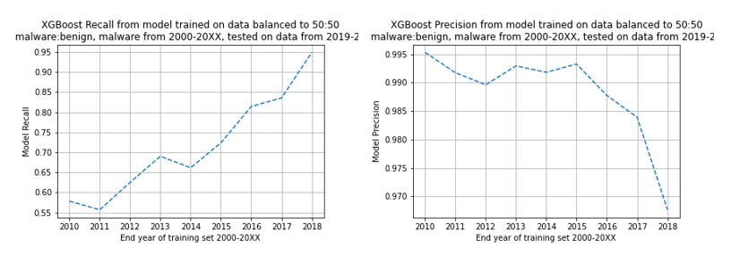
Firstly, note the y-axis on the precision graph – the precision changes nowhere near as much as the recall, where we see around an average of 5% decline in performance per year. The likely reason that the precision changes is the introduction of more malware in the later dated files. What this does unfortunately indicate is that the model will not remain effective for very long; it may need maintaining and updating on new data every year to stay relevant.

Conclusion

The findings above can help contribute to building a more refined model for a specific purpose when it comes to malware identification via PE Headers. Overall, a better understanding of XGBoost’s ability in this domain has been presented, with a slightly deeper dive into what can improve the model’s performance even further.

Although it has been established that a full 60000 strong dataset is not fully necessary, it always makes more sense to feed models as much data as possible. However, the knowledge of how dataset balancing affects precision and recall allows the user to shift model performance in line with their goals. Furthermore, they can vastly reduce training time by simply including the 30 input features listed above.

Further investigation should be made into the feature breakdown, with examination as to why the 30 features listed provide just as much performance, or whether it is even those features specifically and not just a set of 30 random features. Data balancing should also be considered for the time testing, and it may be worth finding a few more training statistics from 2000 onward to further remove any biases from lack of training statistics.

Acknowledgements

Firstly, I would like to thank the whole NCC group for providing the opportunity to tackle this project. In conjunction I would like to thank UCL’s Centre for Doctoral Training in Data Intensive Science for selecting me for the placement. From it I take away invaluable experience using different new technologies, such as AWS’ EC2 instances and VMs, getting to grips with ML via CLI and generally expanding my skills in model evaluation. Explicit thanks go to Tim Scanlon, Matt Lewis and Emily Lewis for help at different phases of the project!

Written by Ewan Alexander Miles.

References

[1] E. Lewis, T. Mlinarevic, A. Wilkinson, Machine Learning for Static Malware Analysis. 10 May 2021. UCL, UK.

[2] E. Raff, J. Sylvester, C. Nicholas, Learning the PE Header, Malware Detection with Minimal Domain Knowledge. 3 Nov 2017. New York, NY, USA.

[3] Y. Liao, PE-Header-Based Malware Study and Detection. 2012. University of Georgia, Athens, GA.

[4] Scikit-learn. Feature importance with a forest of trees. Accessed 6 Dec 2021.

[5] M. Stewart. Guide to Classification on Imbalanced Datasets. 20 Jul 2020. Towards Data Science.